[[TOC]]
DynamoDB Architecture
NoSQL Public Database as a service DBaaS - key/value and document
- no self managed servers or infrastructure
- Manual/Automatic provisioned performance IN/OUT or On-Demand
- Highly resilient across AZs and optionally global
- very fast - single digit milliseconds (SSD based)
- backups, point in time recovery, encryption at rest
- Event-Driven integration - do things when the data changes.
Tables
Think of this as Database Table as a Service. A table is a grouping of items with the same primary key
- simple (Partition) or composite (Partition and Sort)
- primary keys and sort keys must be unique
- none, all, mix or different attributes
- max size of an item is 400kb.
Capacity is measured in speed
- Write = 1WCU = 1kb/second
- Read = 1RCU = 4kb/second
Backups:
- On-Demand - restore to same or cross region
- With or without indexes
- adjust encryption settings
- Point in time recovery (PITR)
- Not enabled by default
- 35 day recovery
- one second granularity
Exam tips:
- NoSQL prefers DynamoDB
- Relational data is not DynamoDB
- Key/Value prefers DynamoDB
- Access via console, CLI, API - NoSQL
- Billed based on RCU, WCU, Storage and features.
DynamoDB Operations, Consistency and Performance
On-Demand - unknown, unpredictable, low admin On-Demand - price per million R or W unites Provisioned, RCU and WCU are set on a per table basis
- every operation consumes at least 1 RCU/WCU
- 1 RCU is 1x4kb read operation per second. If you use 1kb, it rounds up to the 4 and you are charged for that.
- 1 WCU is 1x1kb write operation per second.
- Each table has a burst pool on these (300 seconds)
Query
Can only query on PK or SK values. Try to return as much as you can because you get charged per RCU, so fill it up with 4kb.
Scan
More flexible but it scans through the entire table - you consume all of the items. Lets say you want to scan through a table for all days it rained, you'll scan all the table and only return the ones that it rained on, but the data and capacity was consumed for the discarded, sunny days.
Consistency Model
Lets say you update a DynamoDB table by removing one attribute across the entire table. A leader node takes that write and is now considered consistent, but if there are other storage nodes in other AZs, they are not considered consistent until the change gets replicated from the leader node. This is called 'eventually consistent.'
If someone else reads using the eventually consistent read, they could get some stale data if the node is checked before it is consistent. This is half the cost vs strongly consistent.
WCU Calculation
Writes
Need to store 10 items every second - 10 writes/second with a 2.5k average size Calculate WCU by taking the item size and dividing by 1k and then rounding up to the nearest whole number. 2.5/1 = 2.5 rounded up is 3. 30 WCUs are required.
Reads
Need to retrieve 10 items per second - 10 reads/second with 2.5k average size Calculate RCU by taking the item size and dividing by 4kb and rounding up 2.5/4 = .625 rounded up to 1. 10 RCUs are required. 50% is eventually consistent, 5 required.
DynamoDB Local and Global Secondary Indexes
Query is the most efficient operation in DDB but can only work on 1 PK value at a time.
- and optionally a single or range of Sort Key values
Indexes are alternative views on table data Different Sort Keys (LSI) or Different PK and SK (GSI) Some or all attributes (projection)
A Local Secondary Index (LSI) is an alternative view for at able and must be created with the table.
- 5 LSIs per base table
- Share the RCU and WCU with the table
- Attributes - ALL, KEYS_ONLY & INCLUDE
- Indexes are sparse, only items with the index alternative sort key are added to the index.
A Global Secondary Index (GSI) can be created anytime and there is a default limit of 20 per base table
- have their own RCU and WCUs
- Attributes - ALL, KEYS_ONLY & INCLUDE
GSI's are an alternative view with an alternative PK and SK and they have their own RCU and WCU and can be created anytime.
- any items that have values in the new PK and SK are added - sparse.
GSI are always eventually consistent.
- be careful with projection (KEYS_ONLY, INCLUDE, ALL)
- queries on attributes NOT projected are expensive
- Use GSI's as default, LSI only when strong consistency is required.
- use Indexes for alternative access patterns.
DynamoDB Streams and Lambda Triggers
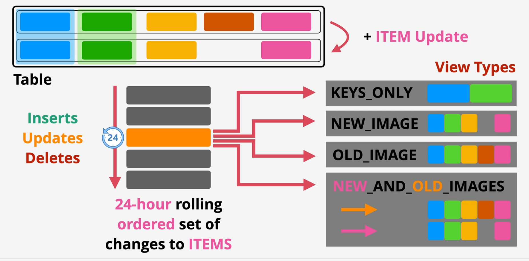
A stream is a time ordered list of item changes in a table.
- this stream is by default a 24 hour rolling window.
- enabled on a per table basis
- Records INSERTS, UPDATES and DELETES
- Different View types influence what is in the stream.
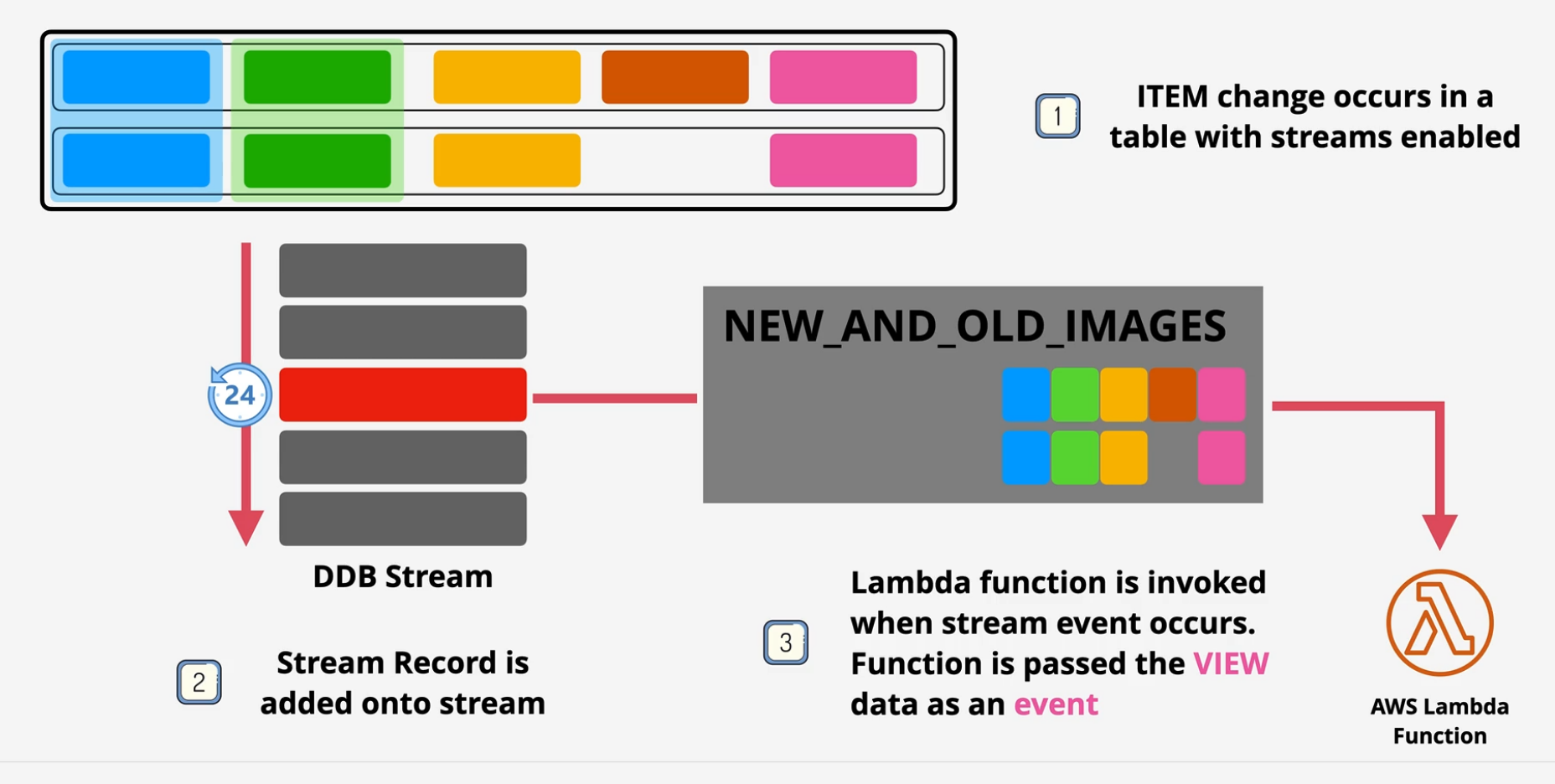
Triggers
- Item changes generate an event
- Event contains the data that has changed
- Action is taken using that data
AWS = Streams + Lambda to implement trigger architecture Usage can be Reporting, analytics, Exports can be data aggregation, messaging or notifications
DynamoDB Global Tables
Multi-master cross-region replication Tables are created in multiple regions and added to the same global table, becoming replica tables.
- Last writer wins is used for conflict resolution
- Reads and writes can occur to any region
- Generally sub-second replication between regions
- eventually consistent
- strongly consistent reads ONLY in the same region as writes.
- provides global HA and global DR/BC
DynamoDB Accelerator (DAX)
Cache miss is when the data is not on the cache, so it reads directly from the source Cache hit is when the data is now on the cache, so it reads from the cache. Separate cache from the DB That's problematic with DynamoDB
With DAX, the same call for data is returned by DAX. DAX either returns the data from the cache or it retrieves it from the database. DAX is built into DynamoDB.
DAX runs within a VPC and needs to be spread across AZs to be resilient. Two different caches
- item cache - results of GetItem
- query cache - parameters and the data
- write through caching.
Primary NODE (Writes) and Replicas (Read) Nodes are HA - primary failure, there is an election to promote another primary node. In-memory cache - scaling = much faster reads, reduced costs. Scale up and scale out (bigger or more) Supports write-through Again, DAX is a public product but needs to be deployed into a VPC and handled as such.
Amazon Athena
Serverless Interactive Querying Service
- ad-hoc queries on data - pay only for what is consumed.
- Schema on read - table like transition
- Original data is not changed - remains on S3
- Schema translates the data -> relational like when read.
- Output can be sent to other services
- source data is read only and fixed. does not change, isn't written to.
THis allows SQL like queries on data without transforming source data with output being sent to visualization tools.
Demo: Amazon Athena
Athena Console
- Log into the AWS console and make sure you're in the N. Virginia region.
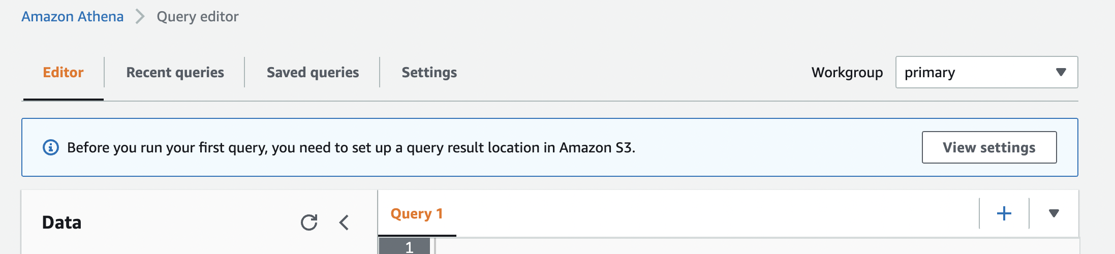
- Navigate to the Athena console and click on query editor
- The first thing we need to do is set up a query result location in S3.
- We'll need to create a bucket first, so let's navigate over to the S3 console.
Create S3 Bucket
- In the S3 console, click create bucket
- Name this something like
babyyoda-athena-demo-query-01, uncheck the boxblock ALL public accessto make the bucket objects public and then create the bucket. - Copy the name of the bucket and head back to the Athena console.
Set up Athena
-
Click on settings and set up the query result location by typing in
s3://and pasting in the bucket name and another forward slash. a. I put in some extra layers here but you can leave the default bucket.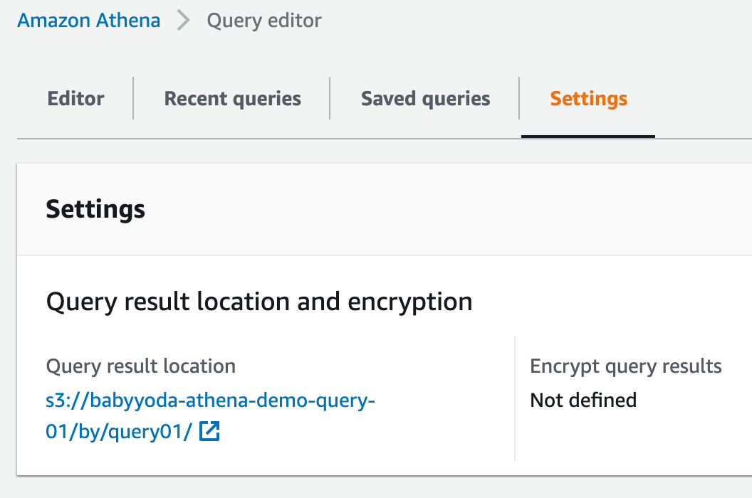
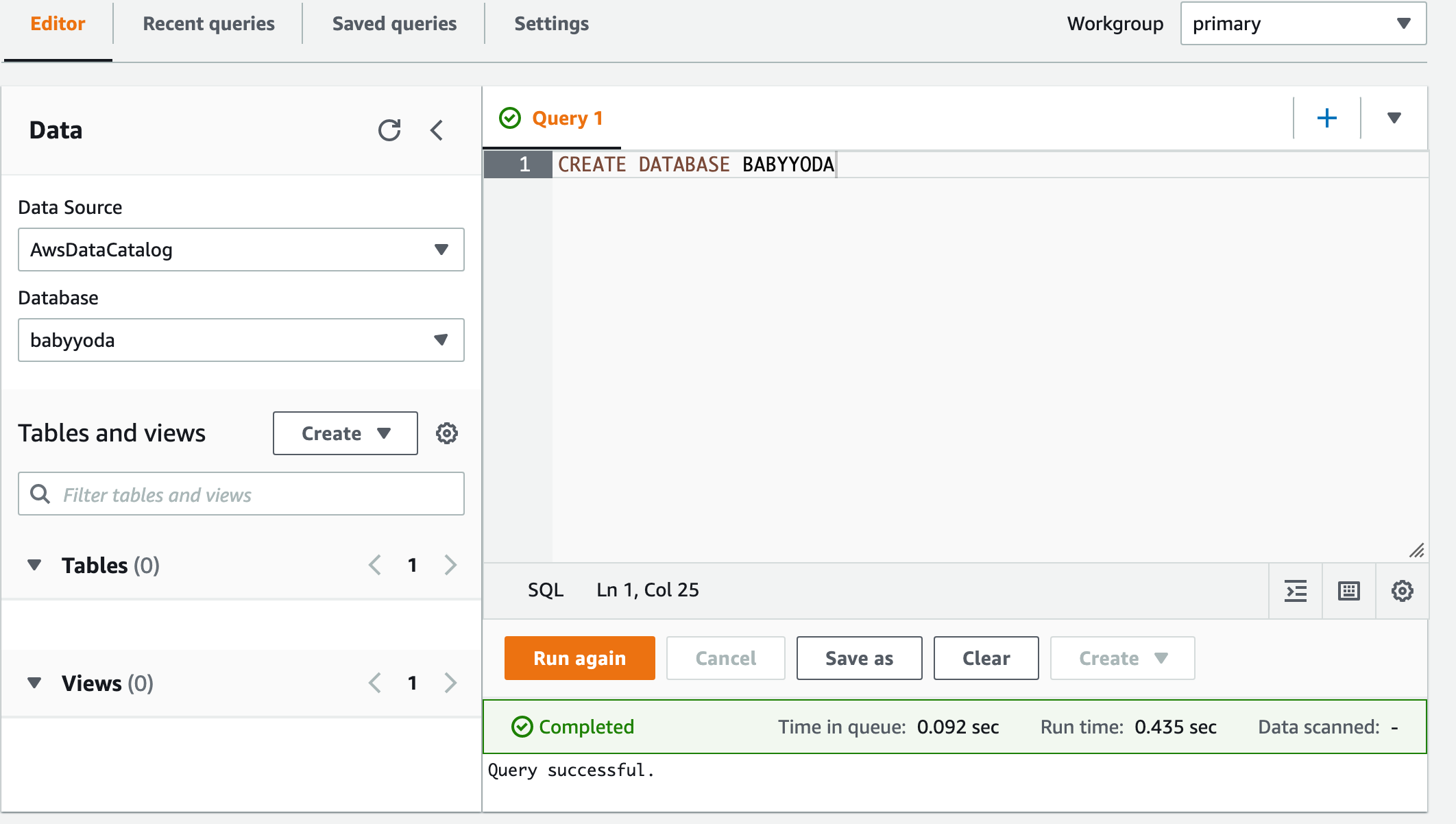
-
Create your default database. You'll need to create the structure in Athena before loading in the source information. Run this command to create the database:
CREATE DATABASE BABYYODA
-
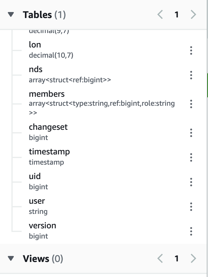
Create the schema for the table. You're not creating the table, just the definition. Copy and paste this into your query window.
CREATE EXTERNAL TABLE planet (
  id BIGINT,
  type STRING,
  tags MAP<STRING,STRING>,
  lat DECIMAL(9,7),
  lon DECIMAL(10,7),
  nds ARRAY<STRUCT<ref: BIGINT>>,
  members ARRAY<STRUCT<type: STRING, ref: BIGINT, role: STRING>>,
  changeset BIGINT,
  timestamp TIMESTAMP,
  uid BIGINT,
  user STRING,
  version BIGINT
)
STORED AS ORCFILE
LOCATION 's3://osm-pds/planet/';
-
There is no data stored in this table. You've built the database and then defined the table structure (schema) that will pull the data from the source
s3://osm-pds/planet/ -
Let's run a test query from the source
SELECT * FROM planet LIMIT 10; -
You should get something as shown below:
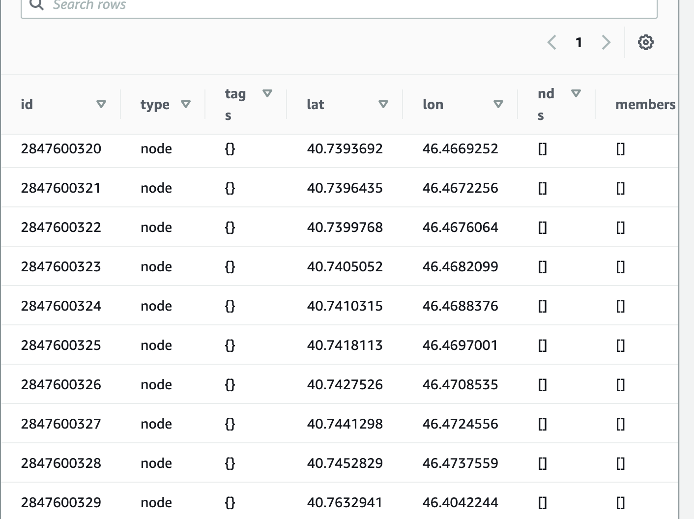
-
What Athena is doing is now reaching out to your SOURCE and then pulling the requested data into your table definition. It's not doing anything more than that.
Finding your Location
- Go to Google Earth.
- Find a location (your house, work, etc) and long click on it. You should bring up the Latitude and Longitude coordinates of that location
a. I used
41.521740, -90.578335:)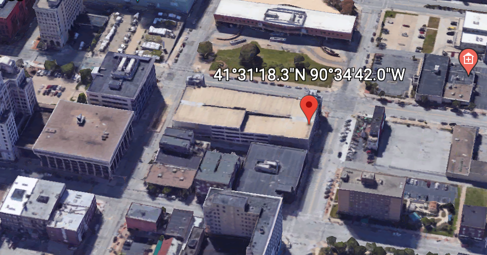
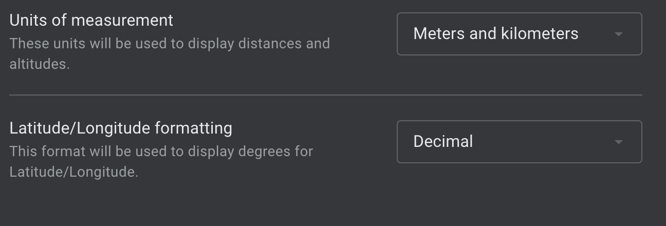
- Click the X to get back to the map.
- Click on settings and change the formatting to decimal.
- What you're going to do is build a box around your search location. We will use this in Athena to gather data from within this square. Click on the shape button at the bottom and draw a shape
- Save this project
- Gather all 4 coordinates.
- 42.249N
- 41.289N
- -87.482W
- -87.267W
- Place these coordinates in the query below:
SELECT * from planet
WHERE type = 'node'
  AND tags['amenity'] IN ('veterinary')
  AND lat BETWEEN 41.546 AND 41.486
  AND lon BETWEEN -90.488 AND -90.484;
Try these too:
SELECT * from planet
WHERE type = 'node'
  AND tags['amenity'] IN ('veterinary')
  AND lat BETWEEN -27.8 AND -27.3
  AND lon BETWEEN 152.2 AND 153.5;
- That queried the entire planet using the location you presented to find any vet offices within that area via Athena.
Clean up
Delete the table - DROP TABLE PLANET
Delete the database - DROP DATABASE BABYYODA
ElastiCache
In-memory database - high performance Two types:
- Redis or memcached...as a service.
- can be used to cache data - for READ HEAVY workloads with low latency requirements
- Reduces database workloads which are expensive
- Can be used to store session data from Stateless Servers
- application needs to know that there is a cache that requires application changes.
Session State Data
Add something to a cart, this goes into ElastiCache.
Redis and Memcached
Memcached
- simple data structures
- no replication
- Multiple nodes - Sharding
- no backups
- multithreaded by design
Redis
- Advanced data structures
- multi-AZ
- Replication (Scale Reads)
- Backup and restore
- Transactions
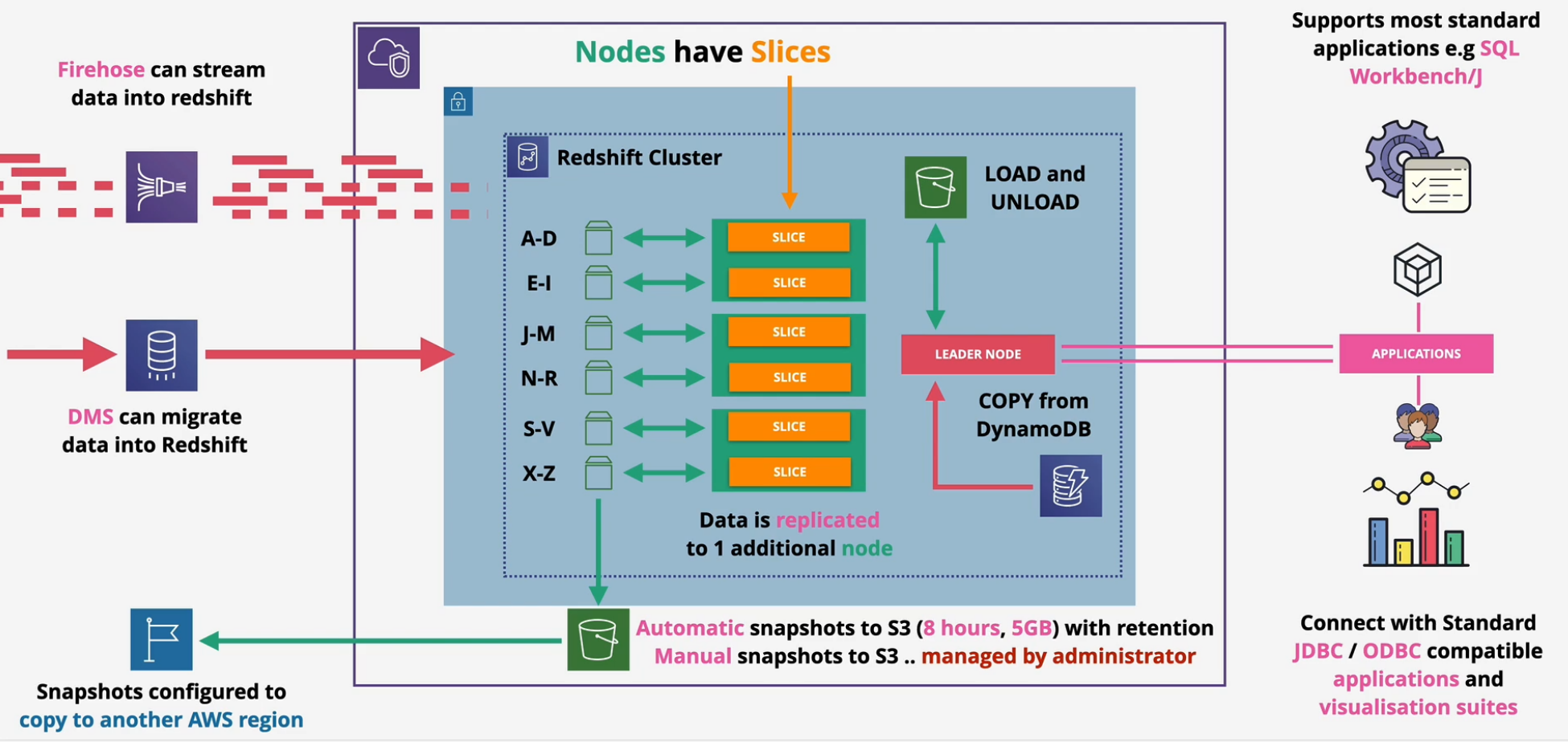
Redshift Architecture
Petabyte-scale Data Warehouse OLAP (Column based) not OLTP (row/transaction) Pay as you use - similar to RDS Direct Query S3 using Redshift Spectrum Direct Query other DBs using federated query. Integrates with AWS tooling such as Quicksight SQL-like interface JDBC/ODBC connections
Uses servers - not serverless Cluster architecture
- one AZ
- leader node - query input, planning and aggregation
- compute node - performing queries of data
VPC Security, IAM Permissions, KMS at rest encryption, CloudWatch Monitoring Redshift Enhanced VPC Routing - VPC Networking
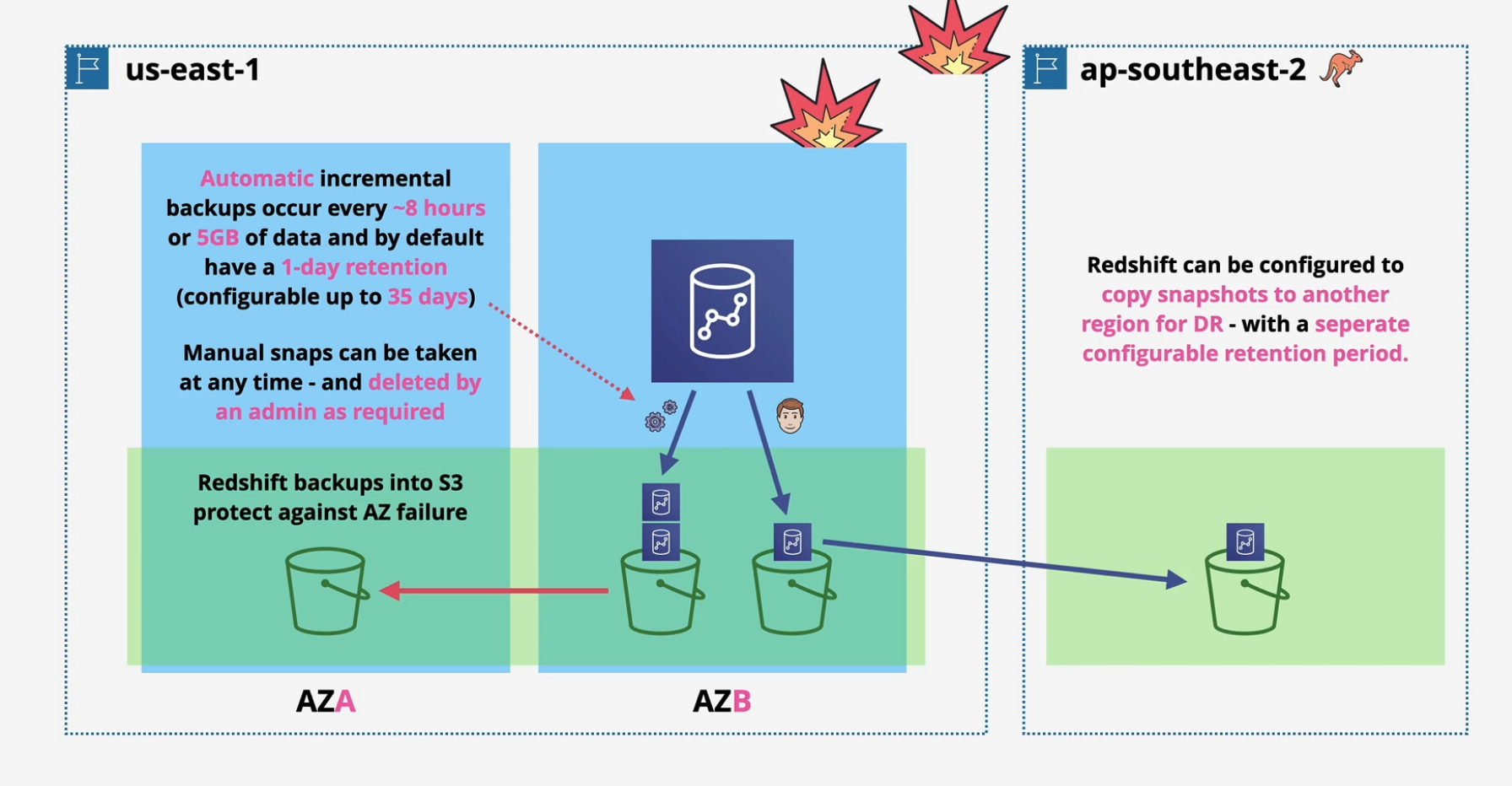
Automatic snapshots to S3 every 8 hours or 5GB. Snapshots can be configured to copy to another AWS region
Redshift DR and Resilience
- Automatic incremental backups occur every 8 hours or 5GB of data (up to 35 days)
- Manual snaps can be taken anytime
- snapshots go into S3 and can be restored across AZs.
- can also copy snapshots into another region for DR.